Micro-C Comparative Analyses

Introduction

Biological questions are seldom answered by analysing single samples in isolation. It is often the case that an experiment aims to make comparisons between two (or more) biological conditions, such as:

1. Untreated wild type vs treatment

2. Wild type vs knockout

3. Normal sample vs tumor

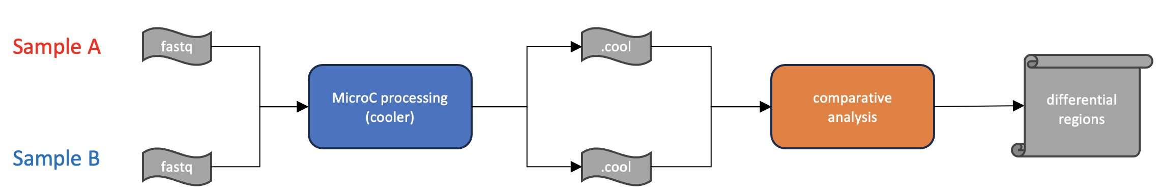
In all cases the goal is to produce a list of differentially interacting regions in one condition relative to the other. The main output for comparative analses is analogous to what is expeected for differential gene expression, where the primary result is a table of regions, the fold change between conditions, and a statistical measure of signficance. For Micro-C, we aim to identify regions of differential interaction directly from the matrix files. See previous steps to generate the required matrices for differential analysis.

Figure 1:

Differential Analysis

Question: How do I perform differential analyses for Micro-C experiments?

Process: Mcool files are first converted to text files of a perferred resolution, and then used as input to the HiCcompare algorithm.

Results: Final results consist of a table of differentially interacting regions, fold change, and measure of statistical signficance.

Files and tools needed:

• .cool, .mcool, .hic, or Hic-Pro files for each replicate and sample condition

• HiCcompare for single-replicate analysis or multiHiCcompare for multiple replicate experiments.

As the design of differential analysis experiments are unique to each biological question, there are multiple possibilites for how the analysis can be set up. A common scenario is to compare two conditions where each condition has two replicates, and is described in the multiHiCcompare vignette. The HiCcompare package also contains functions for conversion of various input files

Interpreting results:

Micro-C differential analysis produces a number of intermediate files in addition to the final results table. There are two main outputs to consider:

1. MD normalization plots

2. Differential regions table

MD is a concept introduced by the HiCcompare developers and is analogous to the Tukey’s mean/difference plot. M corresponds to the log2 fold change between the two conditions, and D is the distance between the two interacting regions. Loess normalization aims to eliminate the bias introduced by the influence of interaction distance on fold change bewteen two conditions. It is often useful to visualize the effect of normalization between conditions to ensure the data is appropriate for downstream difference detection. An example effect of normalization is given below:

Figure 2:

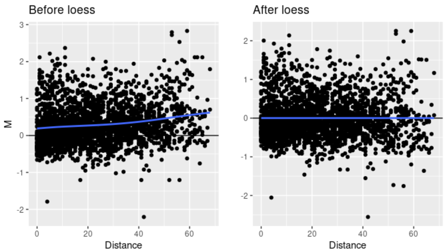
For difference deteciton, the resulting output file is highly similar to what is expected for gene expression studies, where regions are listed and prioritized by a combination of fold change and a measure of statistical signficance. Below is an example output from HicCompare:

chr1	start1	end1	chr2	start2	end2	IF1	IF2	D	M	adj.IF1	adj.IF2	adj.M	mc	A	Z	p.value	p.adj
chr1	10000	11000	chr1	10000	11000	15	1	0	-3.907	14.207	1.056	-3.750	-0.157	7.631	-3.603	0.000	0.736
chr1	16000	17000	chr1	16000	17000	6	2	0	-1.585	5.683	2.112	-1.428	-0.157	3.897	-1.291	0.197	0.863
chr1	17000	18000	chr1	17000	18000	6	3	0	-1.000	5.683	3.167	-0.843	-0.157	4.425	-0.708	0.479	0.904
chr1	22000	23000	chr1	22000	23000	3	1	0	-1.585	2.841	1.056	-1.428	-0.157	1.949	NA	1.000	1.000
chr1	24000	25000	chr1	24000	25000	1	1	0	0.000	0.947	1.056	0.157	-0.157	1.001	NA	1.000	1.000
chr1	27000	28000	chr1	27000	28000	2	2	0	0.000	1.894	2.112	0.157	-0.157	2.003	0.288	0.773	0.904
chr1	28000	29000	chr1	28000	29000	1	1	0	0.000	0.947	1.056	0.157	-0.157	1.001	NA	1.000	1.000
chr1	31000	32000	chr1	31000	32000	4	1	0	-2.000	3.788	1.056	-1.843	-0.157	2.422	-1.704	0.088	0.863
chr1	36000	37000	chr1	36000	37000	2	1	0	-1.000	1.894	1.056	-0.843	-0.157	1.475	NA	1.000	1.000

The most relevant fields from the output will be:

• adj.M – the log fold change in coverage between the two conditions

• p.adj – a p-value, after correction for multiple hypothesis testing, on the statistical signficance of the observed fold change

Considerations:

• Replication – It is generally advisable to have technical replicates for differential analyses, as this will produce more statistically robust results.